Halo Exchange Logic
Introduction
neXtSIM_DG uses MPI to parallelize computation across multiple processes. The total grid is divided into smaller subdomains, each assigned to a different processor. Each processor maintains its own local domain and communicates with neighboring processors through a halo region. Below is an example domain decomposition of the total grid into three domains.
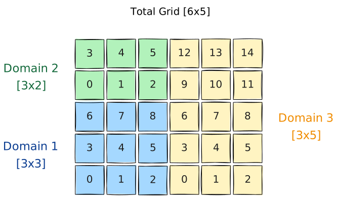
Halo Exchange Overview
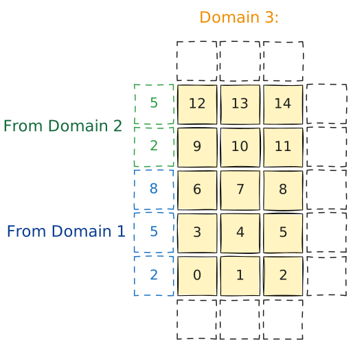
In the following example, we will focus on domain 3. The figure below shows the edge halo
regions surrounding domain 3. The bottom, right and top edges are all on the border.
In this example, we do not use periodic boundaries. So these edges will remain empty. However, the
left edge has two neighbours. The left edge has 5 elements, 3 coming from domain 1 and 2
coming from domain 2.
The domain_decomp tool is designed to generate all the metadata we need to understand which data
to get, which process to get it from and where to store it. To do so, for each neighbour it
generates the following metadata (in file partition_metadata_X.nc, where X is the total
number of processes/domains):
left_neighbours(P)left_neighbour_ids(L)left_neighbour_halos(L)left_neighbour_halo_send(L)left_neighbour_halo_recv(L)
P is the total number of processes/domains and L is the total number of left neighbours
across all domains. In our example the only rank that can have left neighbours is domain 3.
Therefore, left_neighbours would be set as left_neighbours = 0, 0, 2, meaning no left
neighbours for rank 0, no left neighbours for rank 1 and 2 left neighbours for rank 2.
left_neighbour_ids(L) and left_neighbour_halos(L) are used to describe which processes to
get data from, and how much data to fetch, respectively. In this case, they would look like this:
left_neighbour_ids = 0, 1
left_neighbour_halos = 3, 2
This means fetch 3 elements from rank 0, and 2 elements from rank 1. To explain how
left_neighbour_halo_send and left_neighbour_halo_recv work, we first need to understand the
send and recv buffers that are used in Halo.hpp. Each rank produces as send and
recv buffer which it will use to temporarily store the halo data during halo exchange. Each
domain creates it send buffer by forming a 1D buffer from it edges in the order bottom,
right, top and left. This is demonstrated for all domains in the diagram below.
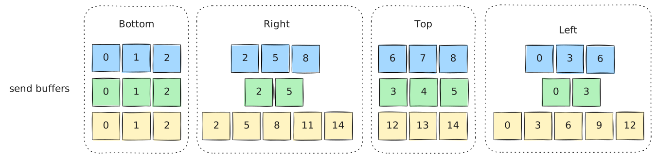
In the previous diagram the edges were grouped to demonstrate how they are produced. But in reality they are stored as a single 1D array as shown in the following figure.
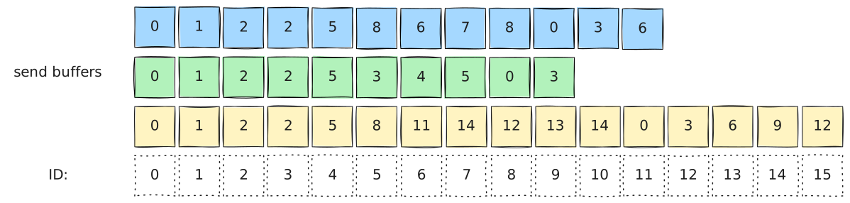
Lets focus on the halo data from domain 1. We know that we need elements 2, 5 and 8.
In Halo.hpp, the send and recv buffers are made accessible through MPI_Win RMA
memory windows. So, we need to know where in rank 0’s send buffer to look for elements
2, 5 and 8. domain_decomp gives us left_neighbour_halo_send which is the
position offset in the send buffer (shown as send pos in the diagram below). So for our example,
left_neighbour_halo_send would be left_neighbour_halo_send = 3, 3. This means that we need
to read 3 elements (left_neighbour_halos[0] = 3) from position left_neighbour_halo_send[0] =
3 in the send buffer of rank 0. Similarly, (by coincidence given this particular
decomposition) the left_neighbour_halo_send send position for domain 2 is also 3.
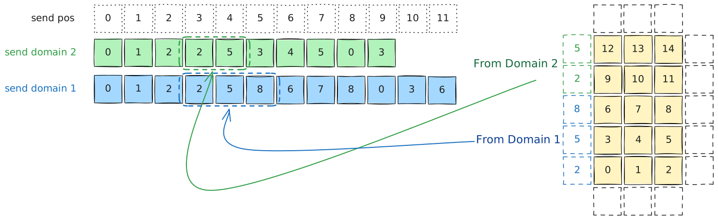
Lastly, we just need to know where to store this data, when we receive it. This is where
left_neighbour_halo_recv comes in handy. left_neighbour_halo_recv is the position offset in
the recv buffer. Like the send buffer, the recv buffer has the same layout, stored in
the order bottom, right, top and left. For this example, left_neighbour_halo_recv
= 11, 14. This tells us to store the 3 elements of domain 1 starting at offset 11 and the 2
elements from domain 2 at offset 14.

The final step of Halo.hpp is to then copy the data from the recv buffer back to the
ModelArray, DGVector or CGVector (depending on the underlying data type).
Notes
Halo.hpp is still under active development. This documentation applies in a similar way for
corner neighbours (currently being implemented). Also, this diagram represents face-centered values
like those in ModelArray HField’s for example. A similar approach is used for
VertexField’s and CGVector’s (currently being implemented).